Using GPE
using_GPE.RmdPrerequisites
You’ll need tabular data with addresses, or “lon” and “lat” columns containing WG84 (Mercator) location coordinates. Examples are a table with the addresses of schools that program beneficiaries attend, or a street or centroid identifying their neighborhoods, or their home addresses if using personal data is allowed.
Geocoding
You can geocode your data (obtain latitude and longitude from addresses) using GPE_geocode(), a function that queries the Google Maps Platform to translate addresses into latitude/longitude coordinates.
Using the Google Maps Platform requires a registered API key. To obtain it, follow instructions from https://developers.google.com/maps/gmp-get-started. Make sure you enable the Geocoding API.
A valid API key is a string of letters and numbers, for example AIjaSyBR76W62lloYPh_c01LYGhCOZuKU6RVW9 -this is not a real ID by the way, just an example. Once you have your key, you can take a data frame with an address column like this one:
## # A tibble: 10 x 3
##    name            address                             level
##    <chr>           <chr>                               <chr>
##  1 EMus 02         Camarones 4351, C1407FMU, CABA      other
##  2 Col La Anuncia… Arenales 2065, C1124AAE, CABA       preschool, primary,…
##  3 EPjs 06         Avda. Eva Perón 7431, C1439BTM, CA… primary
##  4 EPjs 02         Avda. Pte. Manuel Quintana 31/07, … primary
##  5 Col Horacio Wa… Díaz Colodrero 2431, C1431FMA, CABA preschool, primary,…
##  6 EPjc 21         Pinto 3910, C1429APP, CABA          primary
##  7 Casa de la Edu… Boulogne Sur Mer 626, C1213AAJ, CA… primary, secondary
##  8 CFP 06 CIFPA    Avda. Asamblea 153, C1424COB, CABA  secondary
##  9 EI Pulgarcito   Cerrito 572, C1010AAL, CABA         other
## 10 Esc de la Paz   Gral. Venancio Flores 65, C1405CGA… preschool, primary,…
…and add latitude and longitude columns using GPE_geocode, specifying the name of the address column and your Google Maps Platform API key:
key <- "AIjaSyBR76W62lloYPh_c01LYGhCOZuKU6RVW9" # This is not a real API key, you must provide yours

GPE_geocode(schools, address, key)
## # A tibble: 10 x 5
## name address level lon lat
## <chr> <chr> <chr> <dbl> <dbl>
## 1 EMus 02 Camarones 4351, C1407FMU, C… other NA NA
## 2 Col La Anunc… Arenales 2065, C1124AAE, CA… preschool, prima… -58.4 -34.6
## 3 EPjs 06 Avda. Eva Perón 7431, C1439… primary -58.5 -34.7
## 4 EPjs 02 Avda. Pte. Manuel Quintana … primary -58.4 -34.6
## 5 Col Horacio … Díaz Colodrero 2431, C1431F… preschool, prima… -58.5 -34.6
## 6 EPjc 21 Pinto 3910, C1429APP, CABA primary -58.5 -34.5
## 7 Casa de la E… Boulogne Sur Mer 626, C1213… primary, seconda… -58.4 -34.6
## 8 CFP 06 CIFPA Avda. Asamblea 153, C1424CO… secondary -58.4 -34.6
## 9 EI Pulgarcito Cerrito 572, C1010AAL, CABA other -58.4 -34.6
## 10 Esc de la Paz Gral. Venancio Flores 65, C… preschool, prima… -58.4 -34.6Columns with latitude and longitude coordinates are added to the original data frame.
Mapping geocoded data
You’ll need a data frame containing participant data.
GPE includes “participants”, an example data frame with fictional public program beneficiaries:
##   participant_id     group income_bracket
## 1           6494 treatment              6
## 2            409   control              6
## 3           6763 treatment              4
## 4            616   control             10
## 5           4650   control              7
## 6            594   control              8
##                                               address       lon       lat
## 1                              LAVALLE Y PARANA, CABA -58.38835 -34.60277
## 2                        HORTIGUERA Y SANTANDER, CABA -58.44152 -34.63677
## 3                              BAZURCO Y CUENCA, CABA -58.51083 -34.58317
## 4 FIGUEROA ALCORTA, PRES. AV. Y SIVORI, EDUARDO, CABA -58.40110 -34.57915
## 5                     AGUIRRE Y ALVAREZ, JULIAN, CABA -58.43369 -34.59969
## 6                               JUNIN Y LAVALLE, CABA -58.39656 -34.60365
The geographic position of participants and program locations can be plotted, over a basemap, using:
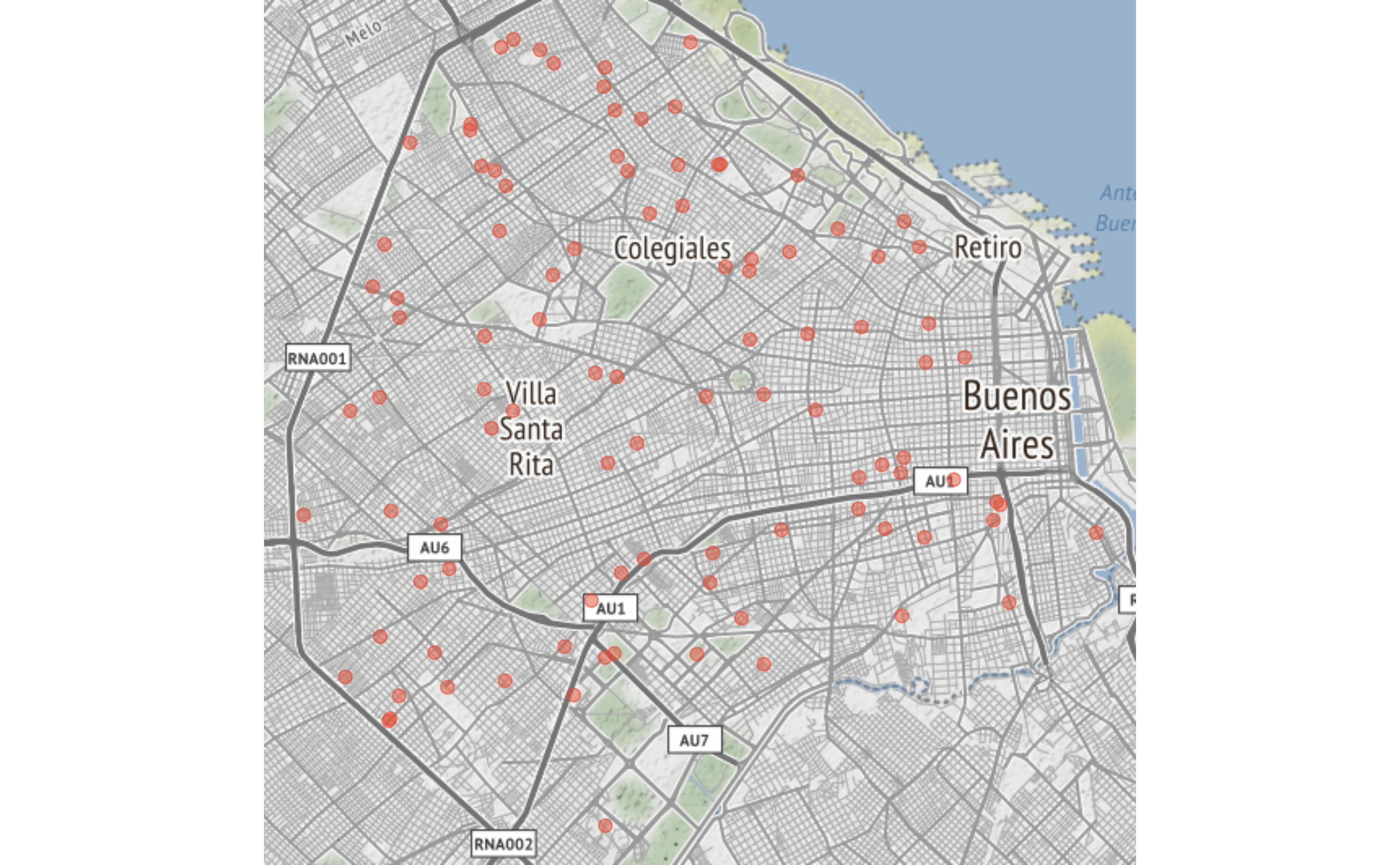
In order for GPE_plot_map() to work, the input data frame must include columns named “lat” and “lon” representing WGS84 coordinates. As previously shown, latitude and longitude columns can be obtained from addresses using GPE_geocode()
In addition, a data frame containing locations -places that participants visit in order to interact with the program, such as training centers, day care providers, etc.- can also be mapped. GPE includes “locations”, an example data frame with fictional public program sites:
## # A tibble: 6 x 4
##   location_id type    lon   lat
##         <dbl> <chr> <dbl> <dbl>
## 1           1 A     -58.4 -34.6
## 2           2 A     -58.4 -34.6
## 3           3 A     -58.4 -34.6
## 4           4 A     -58.4 -34.6
## 5           5 A     -58.4 -34.6
## 6           6 A     -58.4 -34.6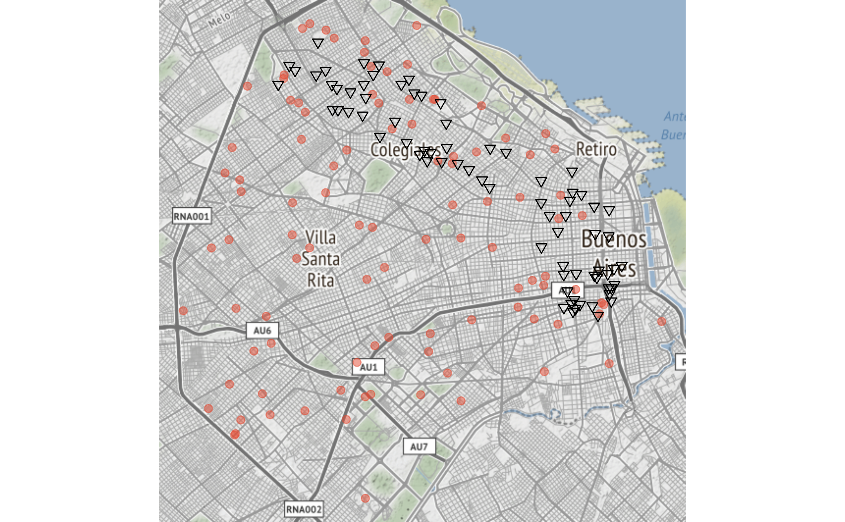
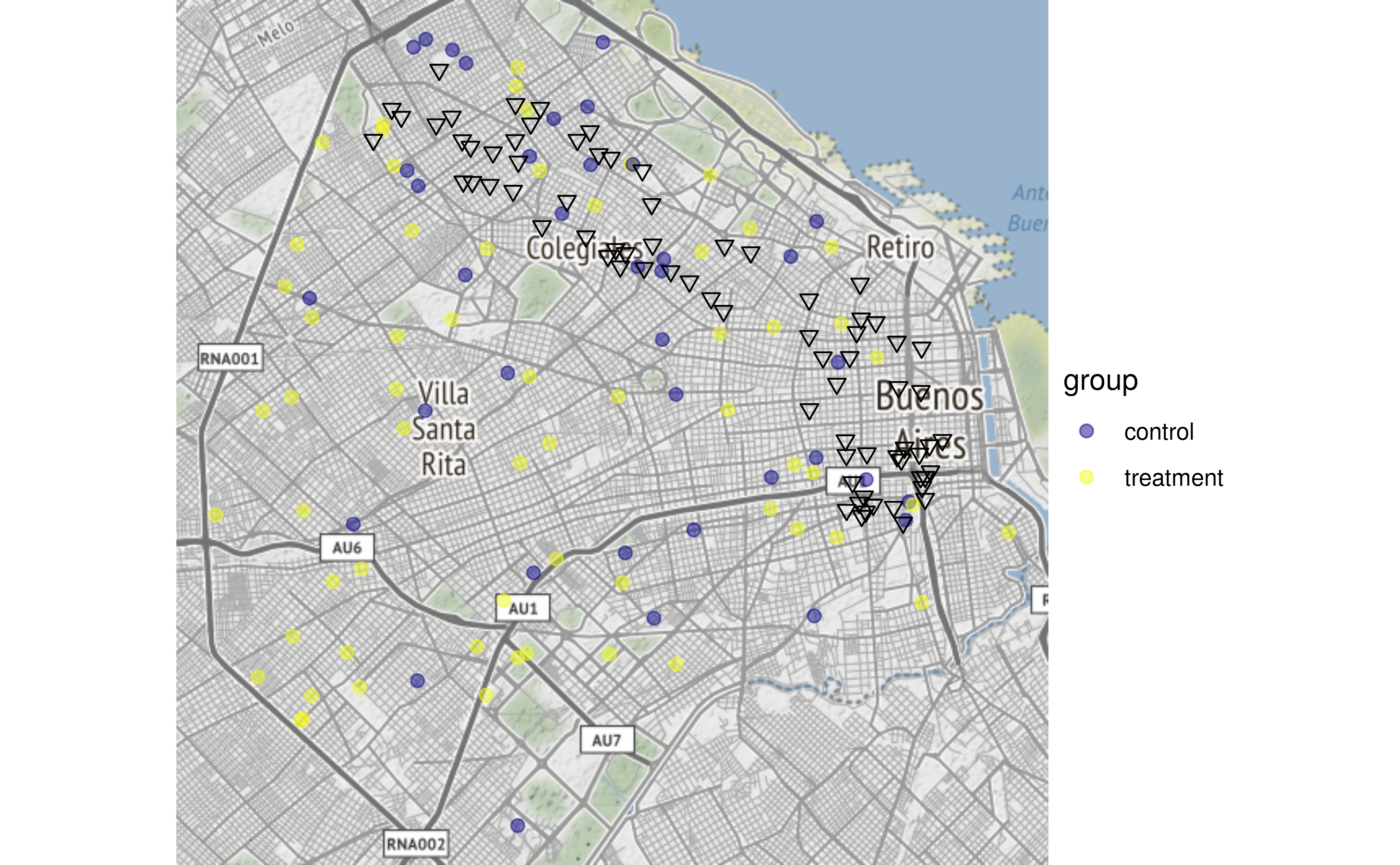
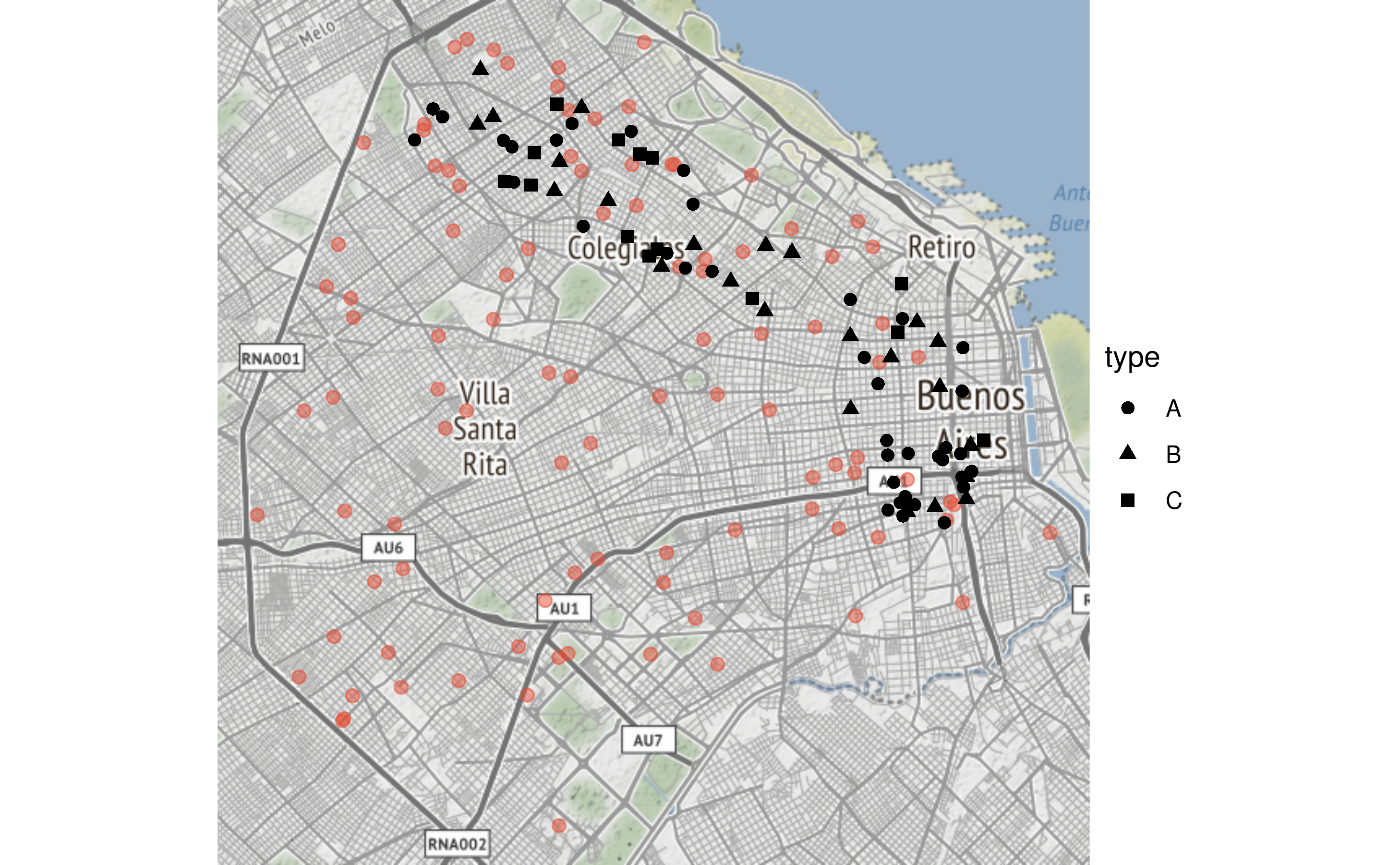
You can also visualize participant attributes by indicating the name of the column that should be used:
The same can be done for location attributes…
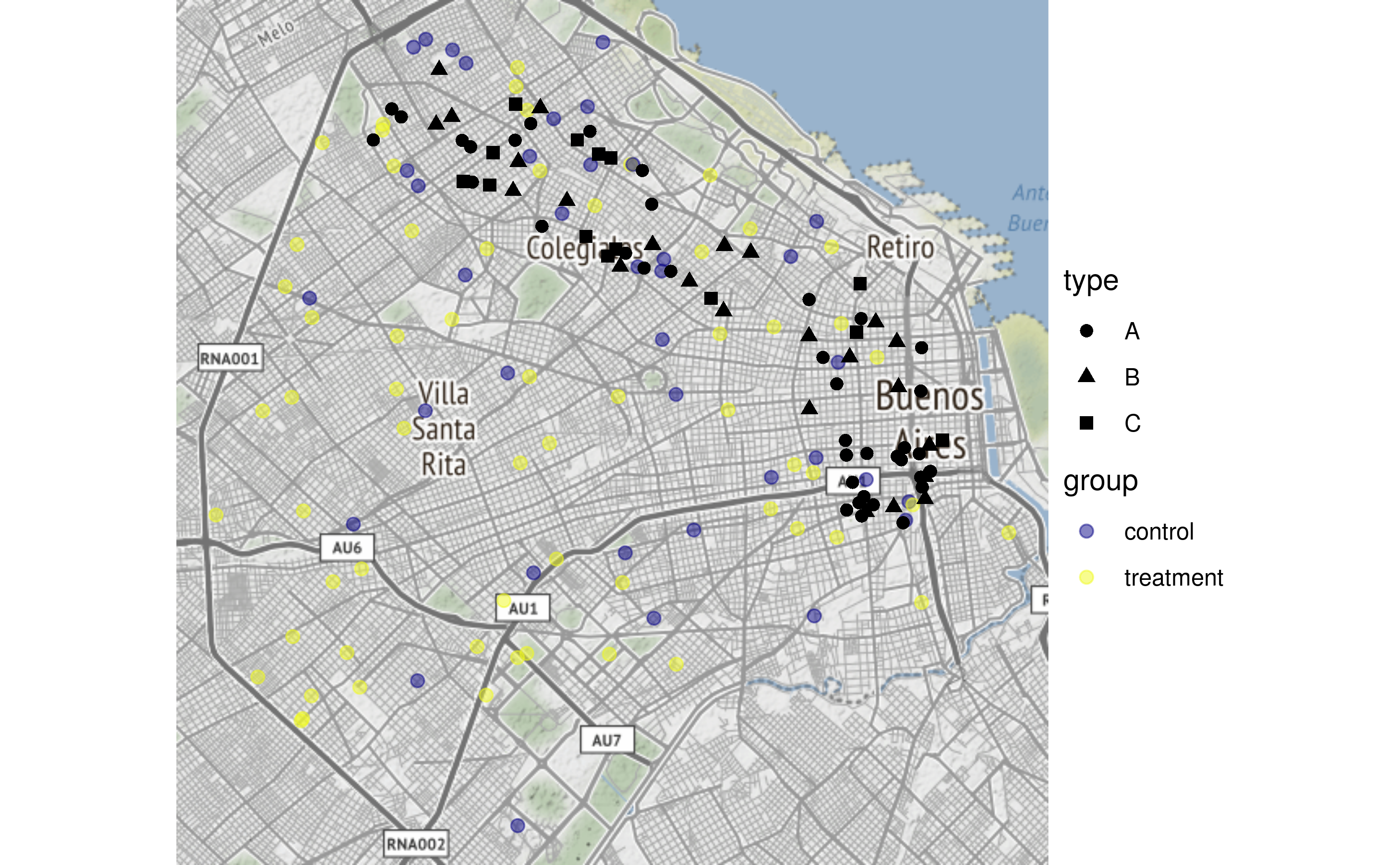
… or both participant and location attributes:
Estimating travel distance and time
Using records of interaction between people and places -representing trips by consumers/beneficiaries to points of sale/access- GPE can estimate time and distance travelled with the Google Maps Platform. As is the case with geocoding, a valid API key is needed to access this service.
GPE provides an example “visits” data frame:
## # A tibble: 10 x 3
##    date       participant_id location_id
##    <date>              <dbl>       <dbl>
##  1 2018-07-22           5786          71
##  2 2018-06-29            804           5
##  3 2018-11-08           6880          76
##  4 2018-03-29            834           6
##  5 2018-05-31           2643          67
##  6 2018-09-18           1694          17
##  7 2018-09-04           4852          26
##  8 2018-08-06           2825           9
##  9 2018-08-16           4522          61
## 10 2018-06-12           3395          61
Trip distance and duration can be obtained using GPE_travel_time_dist(). The function takes as input visits data, as well as the locations and participants data frames that provide the origin and destination coordinates. A valid Google Maps Platform API key is also required. Transport mode can be choose from “transit” (default), “driving”, “walking”, or “bicycling”. Keep in mind that transit routing information is not available for all cities; “driving” and “walking” routing is usually available everywhere.
##          date participant_id location_id time_minutes distance_km    mode
## 1  2018-03-29            834           6     17.38333       2.317 transit
## 2  2018-05-31           2643          67     39.35000       5.511 transit
## 3  2018-06-12           3395          61     39.80000       8.816 transit
## 4  2018-06-29            804           5     36.20000      10.664 transit
## 5  2018-07-22           5786          71     21.75000       2.303 transit
## 6  2018-08-06           2825           9     31.20000       4.363 transit
## 7  2018-08-16           4522          61     40.30000      10.397 transit
## 8  2018-09-04           4852          26     40.81667       5.293 transit
## 9  2018-09-18           1694          17     66.25000      12.231 transit
## 10 2018-11-08           6880          76     55.16667      11.477 transit
Summaries
GPE includes a simple summary function that takes a “visits” data frame, as described before, and returns basic descriptive statistics for
- frecuency of visits, by participant (person)
- frecuency of visits, by location (site)
If the input data frame includes time_minutes and distance_km columns (i.e. as a result of using GPE_travel_time_dist()) the summary will also include basic descriptive statistics for
- travel time, in minutes
- travel distance, in km
For example, given a data frame like
##   participant_id location_id       date time_minutes distance_km    mode
## 1           1080           1 2018-01-20     35.71667      13.230 transit
## 2           1080          23 2018-09-06     61.91667      14.674 transit
## 3           1080          37 2018-06-12     33.11667      12.675 transit
## 4           1080          37 2018-05-02     33.11667      12.675 transit
## 5           1080          51 2018-04-16     51.06667      15.156 transit
## 6           1080          63 2018-11-23     84.15000      12.917 transit
the result is:
## $`visits by participant`
##    Min. 1st Qu.  Median    Mean 3rd Qu.    Max.
##   4.000   5.750   6.500   7.312   8.250  13.000
##
## $`visits by location`
##    Min. 1st Qu.  Median    Mean 3rd Qu.    Max.
##   1.000   3.000   4.000   4.255   6.000  10.000
##
## $`travel time (minutes)`
##    Min. 1st Qu.  Median    Mean 3rd Qu.    Max.
##    6.30   29.00   40.16   40.53   50.27  102.17
##
## $`travel distance (km)`
##    Min. 1st Qu.  Median    Mean 3rd Qu.    Max.
##   0.576   5.122   8.897   9.165  12.921  28.855
Visualization
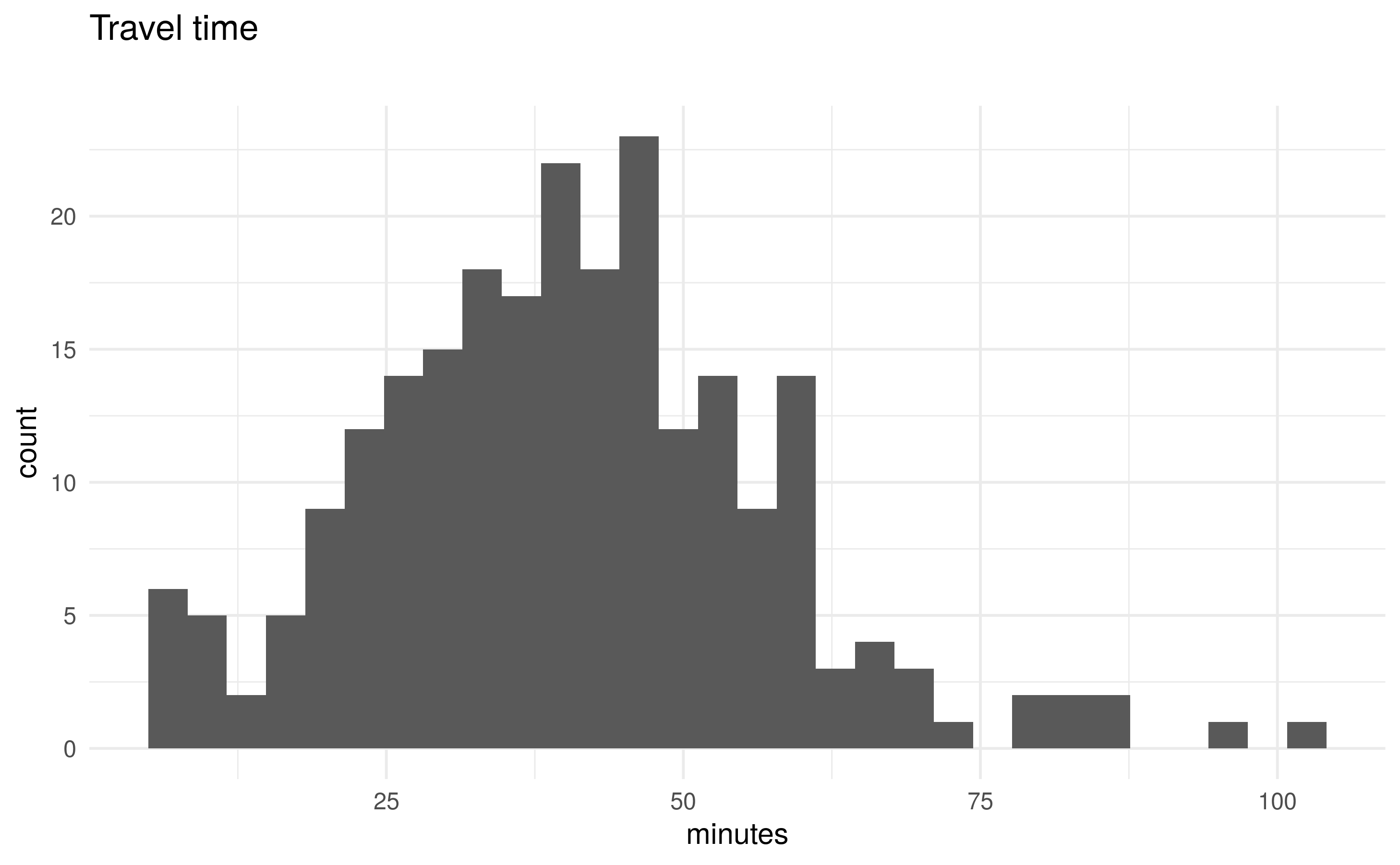
Travel patterns can be visualized using GPE_plot_travel().
The function takes a visits data frame that includes time_minutes and distance_km columns (i.e. as a result of using GPE_travel_time_dist(). By default, it show an histogram with the distribution of travel time (in minutes):
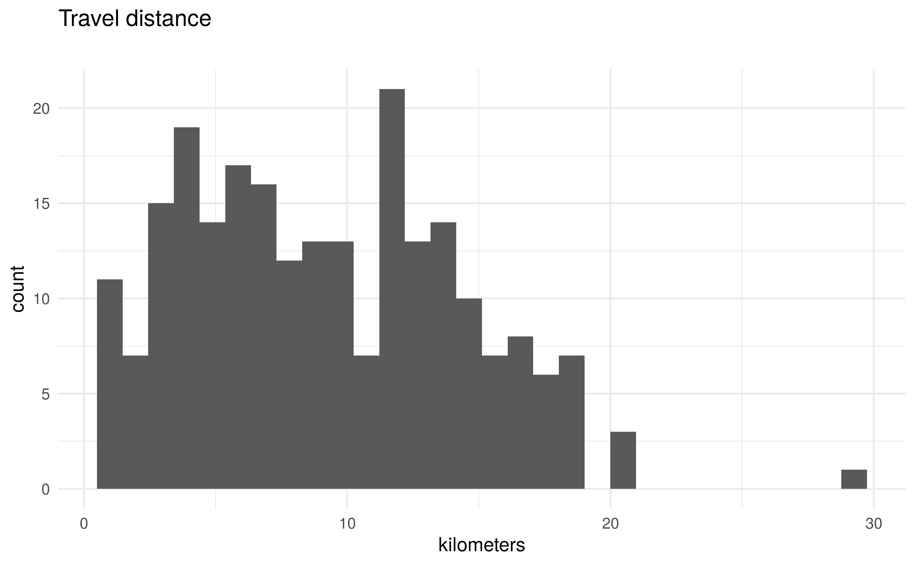
Setting the parameter metric = "time" can be used to used to show travel distance (in kilometers) instead of time:
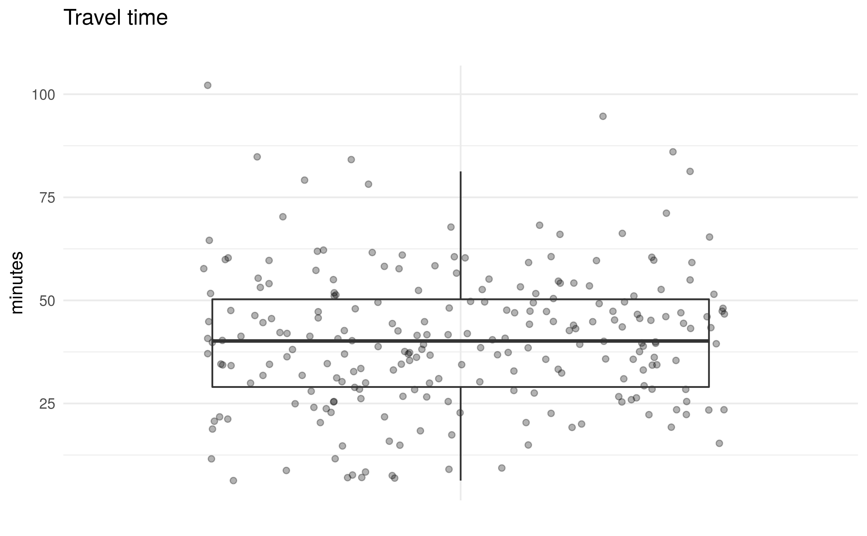
Instead of an histogram, a boxplot can be obtained by setting the parameter plot_type = "boxplot":
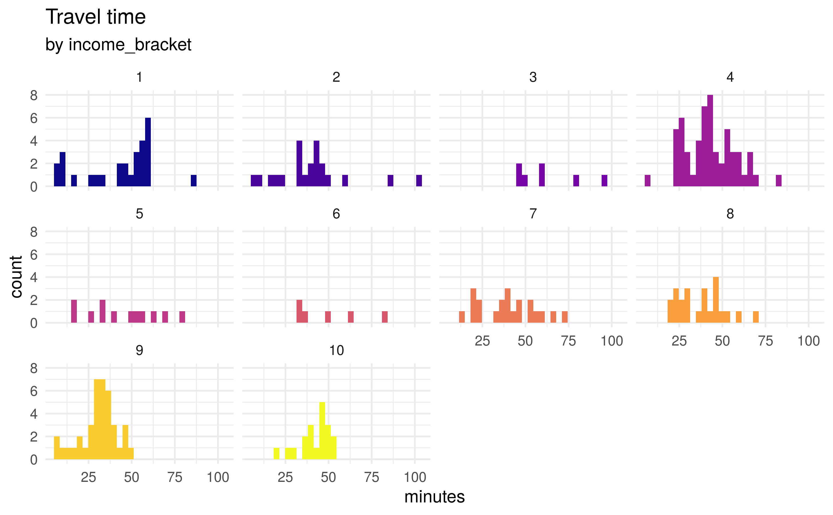
Optionally, an additional data frame can be used as input to merge it with the travel data and plot any of its attributes. This data frame must be contain either participants a locations; that is, besides the attribute to plot it must contain either a “location_id” or a “participant_id” column. When an additional dataframe is used, also specify the name of the column to plot.
For example, to show travel time by participant income level:
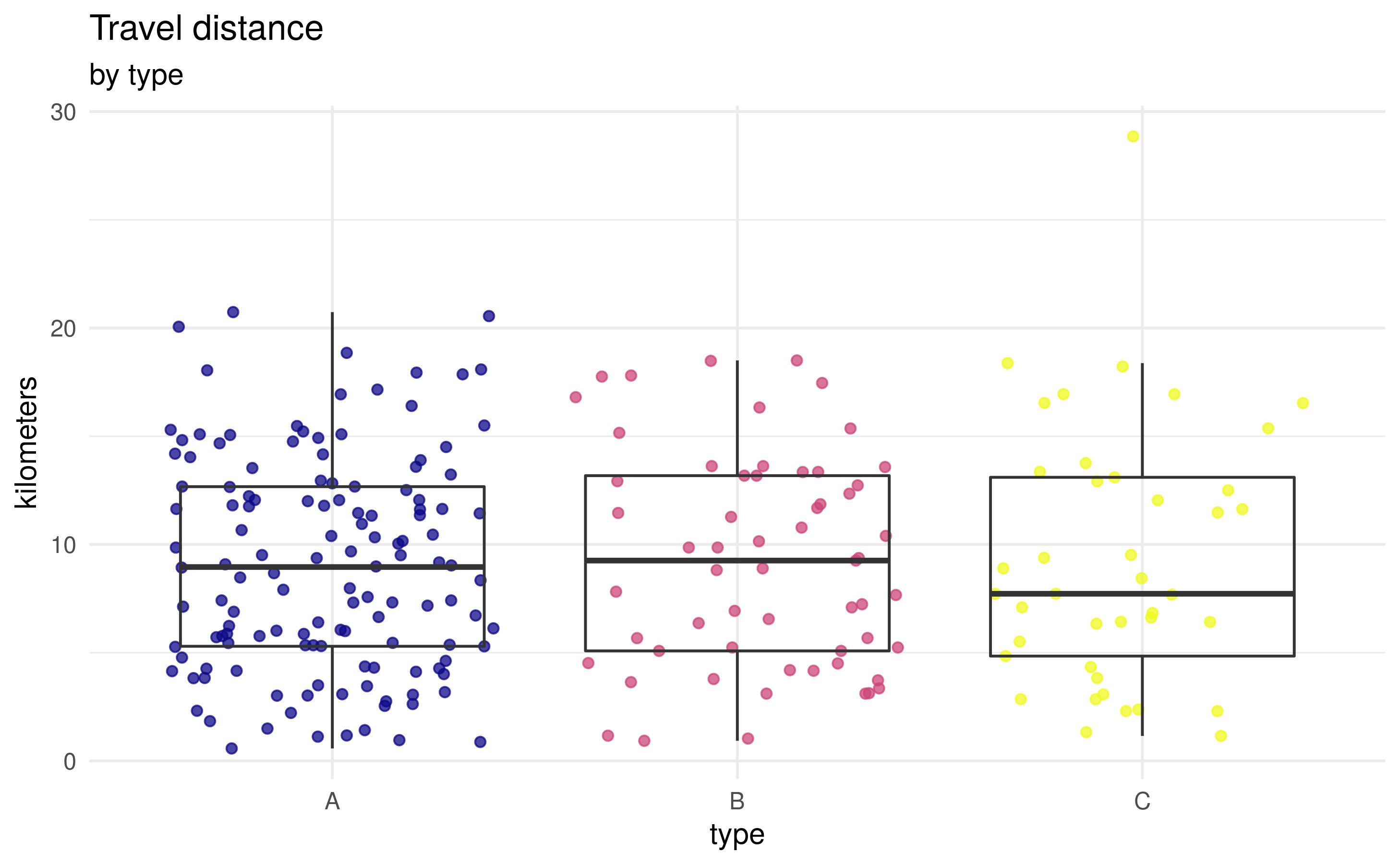
To show travel distance by location type, with boxplots:
GPE_plot_travel(visits_timedist,
                add_data_from = locations, plot_attribute = "type",
                plot_type = "boxplot", metric = "distance")